Spatially Varying Coefficient Models with Spike-and-Slab Group Lasso

2026 Symposium on Data Science and Statistics, Milwaukee, WI USA

Dr. Cheng-Han Yu
Department of Mathematical and Statistical Sciences
Marquette University

2026-04-29

Why Spatially Varying Coefficients (SVC) Models?

• A single global coefficient may mask or distort spatially heterogeneous relationships.

• SVC models let regression effects change with location: \beta_j(s), not a single \beta_j (Gelfand et al. 2003; A. Stewart Fotheringham, Brunsdon, and Charlton 2002).

Published SVC applications show this need in geostatistics.

Air pollution (Hamm et al. 2015)

Forestry (Babcock et al. 2015)

Hydrology (Roksvåg, Steinsland, and Engeland 2022)

Spatially varying coefficient models are not only a theoretical idea. Smooth coefficient surfaces already appear in real geostatistical applications. For example, Hamm and coauthors mapped spatially varying calibration slopes for PM10 across Europe. Babcock and coauthors showed smoothly varying LiDAR effects in forest biomass modeling. Roksvag and coauthors used Gaussian random field coefficient surfaces in runoff modeling. These examples motivate our focus on learning beta surfaces directly, not only fitting responses.

Why Selection Matters in SVC Models

Statistical question: which predictors truly need a spatially varying coefficient surface?

• Not every predictor needs a full spatial coefficient surface.

Example. In a county-level diabetes analysis, population density was significant in the model but locally positive in only 0.7% of counties (Hipp and Chalise 2015).

Why Selection Matters in SVC Models

If \beta_j(s) = 0 for all s but x_j is included, but the model tries to estimate a coefficient surface that does not truly exist or scientific meaningful:

• Estimation (Hastie, Tibshirani, and Friedman (2009); Sestelo et al. (2016))
  • Fit random noise instead of real signal
  • Spatial smoothing can turn noise into a fake-looking spatial pattern
  • Uncertainty in other coefficient surfaces may increase
  • Collinearity with useful predictors can make important effects harder to estimate

• Prediction (Hastie, Tibshirani, and Friedman (2009); Ishwaran and Rao (2005))
  • Increase prediction variance
  • Reduce out-of-sample predictive accuracy

This slide should make the selection need concrete. It is not enough to say spatial effects can vary. We also need to avoid estimating unnecessary coefficient surfaces. The diabetes example is useful because population density was globally significant, but its local effect was absent in most counties. - The predictor contributes little additional signal after accounting for other variables.

• A full spatially varying coefficient surface is unlikely to improve model performance.

Why Selection Matters in SVC Models

If \beta_j(s) = 0 for all s but x_j is included, but the model tries to estimate a coefficient surface that does not truly exist or scientific meaningful:

• Interpretation (Gelfand et al. (2003); Greve and Fischl (2018); Brodoehl et al. (2020))
  • Misread as scientific evidence
  • Suggest that predictor j matters in some locations when it does not
  • Apparent spatial regions of importance may be false positives

• Computational
  • More parameters must be estimated
  • Slower MCMC and longer computation

Gap in Existing Methods

Standard selection

✅ sparse predictors
❌ spatially varying effects

Lasso and group lasso select variables or groups, but their standard forms use global coefficients (Tibshirani 1996; Yuan and Lin 2006).

SVC / GWR

✅ spatially varying effects
❌ automatic surface selection

SVC and GWR estimate location-specific or process-based coefficient variation (Gelfand et al. 2003; A. Stewart Fotheringham, Brunsdon, and Charlton 2002).

Penalized spatial methods

✅ shrinkage / local selection
❌ posterior uncertainty as a default output

Geographically weighted lasso is optimization based (Wheeler 2009).

Bayesian SVC selection

✅ model uncertainty
❌ a general scalable surface-selection template

Existing Bayesian SVC selection is often model- or application-specific (Reich et al. 2010; Shang and Clayton 2012; Boehm Vock et al. 2015; Mu et al. 2021).

Need: spatial flexibility + predictor-level surface selection + Bayesian uncertainty quantification.

Keep this as a gap slide, not a method slide. The message is that each existing class gives part of the solution. The novelty is the combination we need for SVC surface selection.

SSGL-SVC: Our Solution

• Represent each spatially varying coefficient surface with a low-rank basis expansion

\beta_j(s) = \sum_{h=1}^H B_h(s)\alpha_{jh}, \quad j = 1, \dots, p

• Apply spike-and-slab group lasso shrinkage to the basis coefficients for each predictor

\boldsymbol{\alpha}_j = (\alpha_{j1}, \ldots, \alpha_{jH})^\top

• Selection operates at the predictor-surface level (not local regions)

  • keep predictor j if its coefficient surface is supported by the data
  • shrink the entire surface toward zero if the predictor is weak

• The result is a scalable Bayesian SVC model with interpretable spatial surfaces and posterior uncertainty

The previous slide identified the methodological gap. This slide presents the proposed solution. Instead of estimating one coefficient at every location, SSGL-SVC first represents each coefficient surface using a lower-dimensional basis expansion. The model then applies spike-and-slab group lasso shrinkage to the basis coefficients associated with each predictor. This means selection is made at the predictor-surface level. If a predictor has meaningful spatially varying effects, its surface is retained. If the predictor is globally weak, the entire surface is shrunk toward zero. This gives us a model that is spatially flexible, easier to interpret than an unregularized SVC model, and more scalable because selection happens after reducing the raw spatial dimension.

SSGL-SVC: Basis Representation and Low-Rank Design

• A separate coefficient at every location for every predictor

• Gaussian process dimension grows like p \times n location-specific coefficients

SSGL-SVC: Basis Representation and Low-Rank Design

• Approximate each coefficient surface with H basis functions, where H \ll n

• Predictor x_j get one coefficient block (\eta_{j1}, \dots, \eta_{jH})

Dimension changes from pn location-level coefficients to pH grouped basis coefficients

SSGL-SVC: Basis Representation and Low-Rank Design

Turn SVC Into a Grouped Regression

y_i = \alpha_0 + \sum_{j=1}^{p} x_{ij}\,\beta_j(s_i) + \varepsilon_i, \qquad \varepsilon_i \stackrel{iid}{\sim} N(0,\sigma^2), \qquad i = 1, \dots, n

\beta_j(s) = \mathbf{B}(s)^\top \boldsymbol{\eta}_j, \qquad \mathbf{B}(s) = \big(B_1(s),\ldots,B_H(s)\big)^\top

\boldsymbol{\eta} = \big(\boldsymbol{\eta}_1^\top,\ldots,\boldsymbol{\eta}_p^\top\big)^\top, \qquad \mathbf{y} = \alpha_0\mathbf{1}_n + \mathbf{Z}\boldsymbol{\eta} + \boldsymbol{\varepsilon}

\mathbf{Z} = [\mathbf{Z}_1\ \cdots\ \mathbf{Z}_p], \qquad \mathbf{Z}_j = \operatorname{diag}(x_{1j},\ldots,x_{nj})\,\mathbf{\Phi},

where \mathbf{\Phi}_{n\times H} = \left( \mathbf{B}(s_1)^\top, \mathbf{B}(s_2)^\top \dots, \mathbf{B}(s_n)^\top \right)^\top

• Represent each spatially varying coefficient surface by a shared low-rank basis expansion rather than a separate coefficient at every observed location.
• Use the same basis functions across predictors, so predictor j contributes one block of coefficients \boldsymbol{\eta}_j \in \mathbb{R}^H.
• This turns the SVC problem into a grouped linear model with only pH unknown basis coefficients instead of pn location-specific parameters.
• The low-rank design improves scalability, stabilizes estimation, and yields smooth coefficient maps through the basis functions. The key structural idea is low-rank basis expansion. Each predictor-specific coefficient surface is written using the same shared basis, so every predictor corresponds to one coefficient block. This reduces the raw dimension from location-specific parameters to grouped basis coefficients and makes the model much more scalable.

SSGL-SVC: Basis Representation and Low-Rank Design

\boldsymbol{\eta} = \big(\boldsymbol{\eta}_1^\top,\ldots,\boldsymbol{\eta}_p^\top\big)^\top, \qquad \mathbf{y} = \alpha_0\mathbf{1}_n + \mathbf{Z}\boldsymbol{\eta} + \boldsymbol{\varepsilon}

\mathbf{Z} = [\mathbf{Z}_1\ \cdots\ \mathbf{Z}_p], \qquad \mathbf{Z}_j = \operatorname{diag}(x_{1j},\ldots,x_{nj})\,\mathbf{\Phi},

• Use the same basis matrix \mathbf{\Phi}_{n\times H} for all predictors; multiply by each covariate to form grouped design blocks

SSGL-SVC: Spike-and-Slab Group Lasso Prior

Basis expansion improves scalability, but does not solve predictor selection.

SSGL-SVC: Prior Setting

• Spike-and-Slab Group Lasso (Multivariate Laplace)

p(\boldsymbol{\eta}\mid \boldsymbol{\gamma}) = \prod_{j=1}^{p}\Big[(1-\gamma_j)\,\Psi(\boldsymbol{\eta}_j\mid \lambda_0) + \gamma_j\,\Psi(\boldsymbol{\eta}_j\mid \lambda_1)\Big], \quad \lambda_0 > \lambda_1 > 0

\Psi(\boldsymbol{\eta}_j\mid \lambda) \propto \exp\big(-\lambda \lVert \boldsymbol{\eta}_j \rVert_2\big)

\eta_j \mid \tau_j,\sigma^2 \sim N(\bm{0},\sigma^2\tau_j\hbox{\bf I}_H), \qquad \tau_j\mid \gamma_j \sim Ga\!\left(\frac{H+1}{2},\frac{\lambda_{\gamma_j}^2}{2}\right),\qquad \lambda_{\gamma_j}= \begin{cases} \lambda_0,&\gamma_j=0,\\ \lambda_1,&\gamma_j=1. \end{cases}

• The posterior inclusion probability (PIP) P(\gamma_j=1\mid\mathbf y) summarizes the posterior probability that predictor x_j has a non-negligible (spatially varying allowed) coefficient surface.

• Other priors \sigma^2\sim IG(a_\sigma,b_\sigma), \quad \gamma_j\mid \theta \sim \mathrm{Bernoulli}(\theta), \quad \theta \sim \mathrm{Beta}(a,b)

• Treat each predictor-specific coefficient surface as one group, so selection is performed at the predictor level, not basis by basis.
• If \gamma_j = 0, the spike component with large \lambda_0 strongly shrinks the whole surface \beta_j(\cdot) toward zero.
• If \gamma_j = 1, the slab component with smaller \lambda_1 allows a non-negligible and spatially varying effect surface.
• The shared inclusion probability \theta provides multiplicity control and yields posterior inclusion probabilities as natural summaries of selection uncertainty.
• This prior combines smooth coefficient estimation, group sparsity, and explicit model uncertainty quantification in one Bayesian framework. The prior acts on whole predictor blocks. The spike component shrinks an entire coefficient surface toward zero, while the slab component keeps a predictor active and allows spatial variation. This is the core reason the method can do predictor-level selection and still estimate smooth coefficient maps.

Posterior Computation

• A Gibbs sampler is developed.

• Posterior draws

  • \boldsymbol{\eta} from normal
  • \sigma^2 from inverse gamma
  • \boldsymbol{\tau} from generalized inverse Gaussian
  • \boldsymbol{\gamma} from Bernoulli
  • \theta from beta

• Derived coefficient surfaces \beta_j(s)=\mathbf{B}(s)^\top \boldsymbol{\eta}_j

Low-rank basis expansion makes each update depend on pH, not pn, spatial coefficients.

Low-rank spatial representations are a common strategy for scaling spatial models (Banerjee et al. 2008; Guhaniyogi et al. 2022).

Do not derive the full conditionals. The audience needs to know the computation is posterior sampling, and that the basis representation is what makes the grouped selection problem computationally manageable.

• Gibbs style posterior sampling with structured block updates
• Update coefficient blocks, shrinkage parameters, inclusion indicators, and variance terms
• Basis reduction keeps the computation manageable
• Designed for practical spatial data analysis I will not go into full conditional details here, but the main computational strategy is a Gibbs style sampler with block updates. The basis representation is important not only for modeling but also for computation, because it reduces the effective dimensionality of the spatial problem.

Simulation Design

Component	Design
Sample size	n=1000, 2000, 10000
Predictors	p=5,7,10
Metrics	prediction error, surface MSE, selection accuracy, time

• Basis-based
  • Gaussian-SVC: No shrinkage, and ridge-type prior on each basis coefficient
  • BSGL-SVC (Continuous Bayesian spatial group lasso) (Zhan et al. 2026): Continuous shrinkage with no spike-and-slab
  • GGP-GAM (Geographical Gaussian process generalized additive model) (Comber, Harris, and Brunsdon 2024): frequentist equivalent of BSGL-SVC
• Nonbasis-based
  • MGWR (Multiscale geographically weighted regression) (A. Stewart Fotheringham, Yang, and Kang 2017): non-basis frequentist benchmark

Use this as a clean design table. Do not spend time on all simulation details. The design should signal that the comparisons target both estimation and selection.

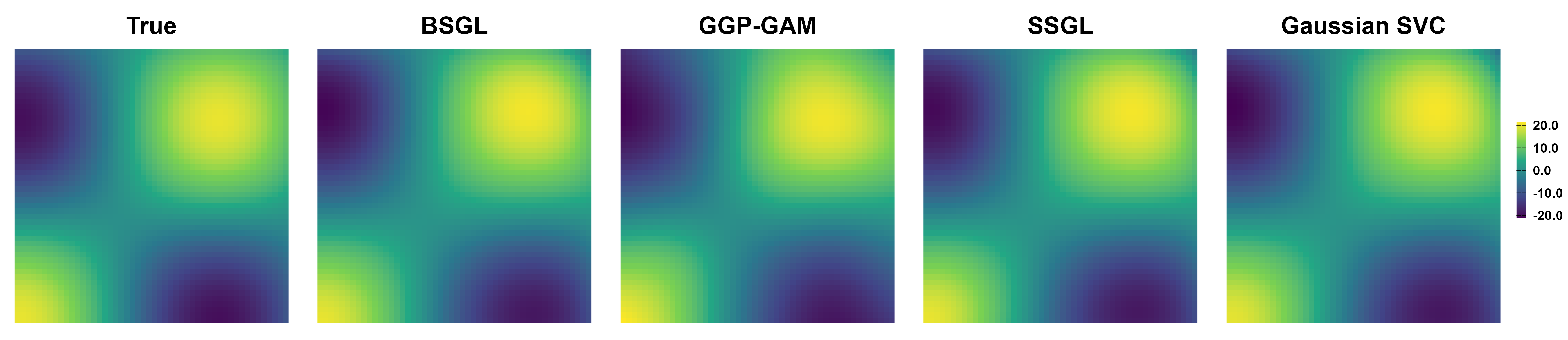
Simulation Results: Surface Recovery

All competing methods recover the main spatial patterns of active predictors with large signals

Selection alone is not enough in this problem. We also need good recovery of the spatial coefficient surfaces. This slide shows that the proposed method not only identifies relevant predictors, but also reconstructs their spatial patterns well, while shrinking irrelevant effects toward zero.

Simulation Results: Variable Selection

SSGL-SVC separates signal predictors from noise predictors more sharply than continuous shrinkage alone, BSGL-SVC and Gaussian-SVC.

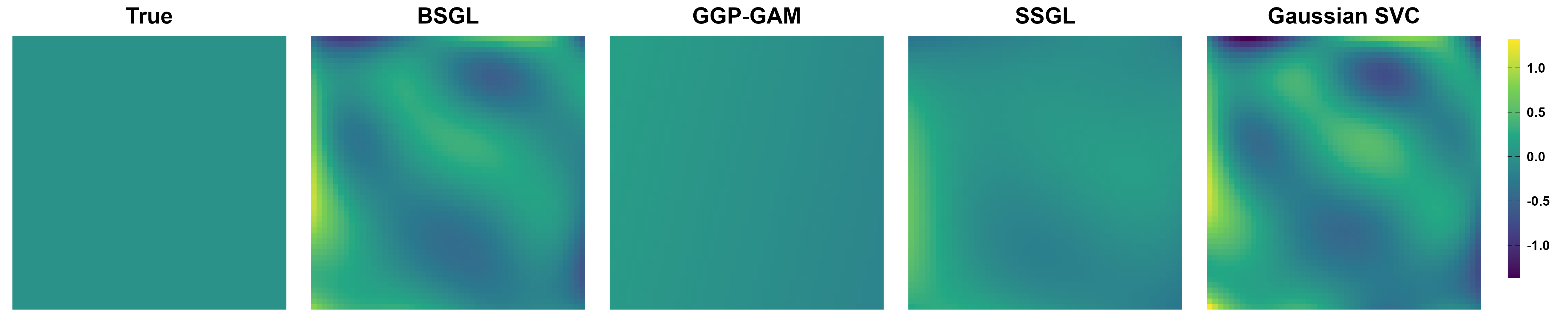
• GGP-GAM seems to work well, but . . .

Here the main message is that the proposed method distinguishes signal predictors from noise predictors more effectively across the simulation settings we considered. I would emphasize the overall separation and stability rather than any single number on this slide.

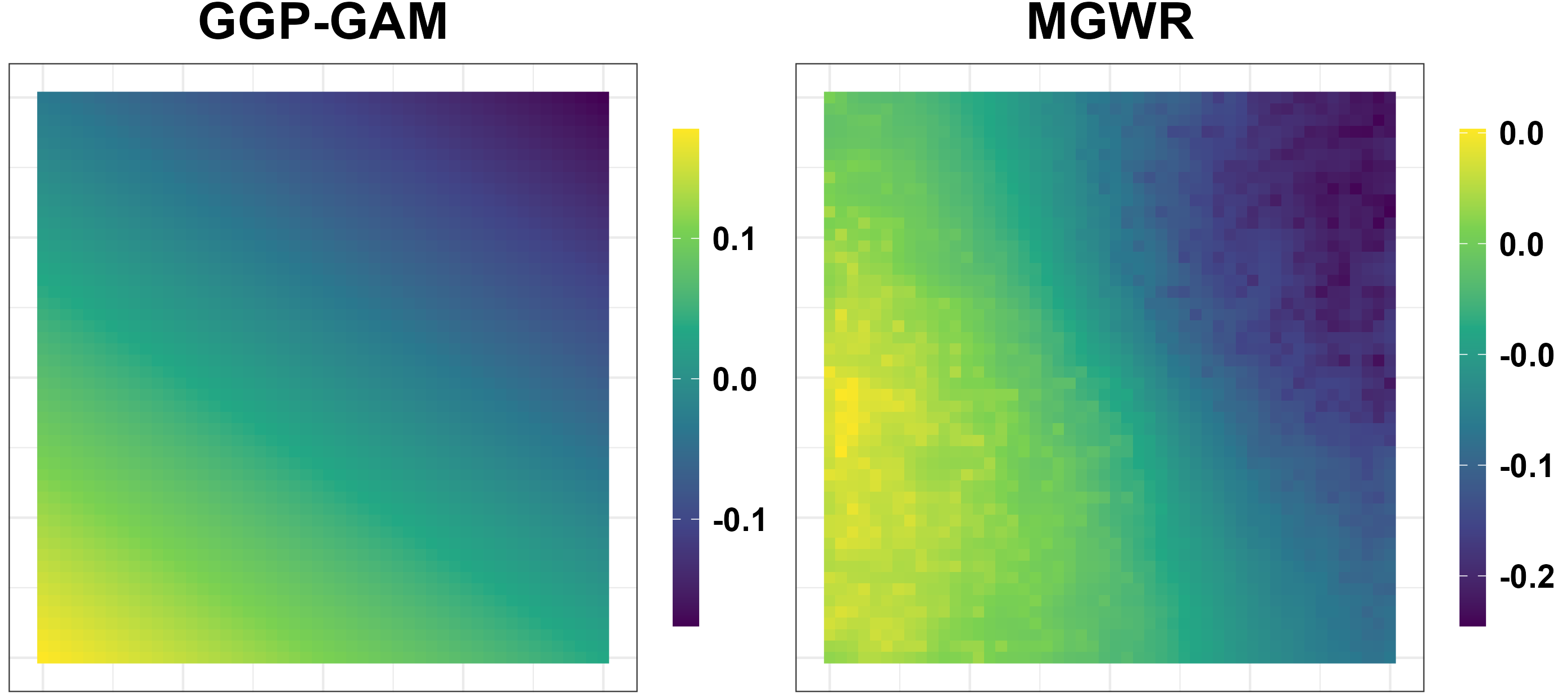
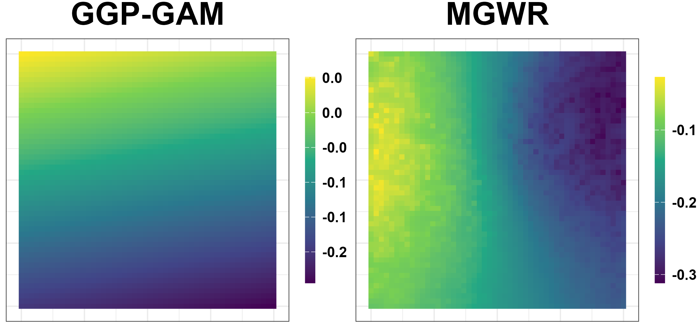
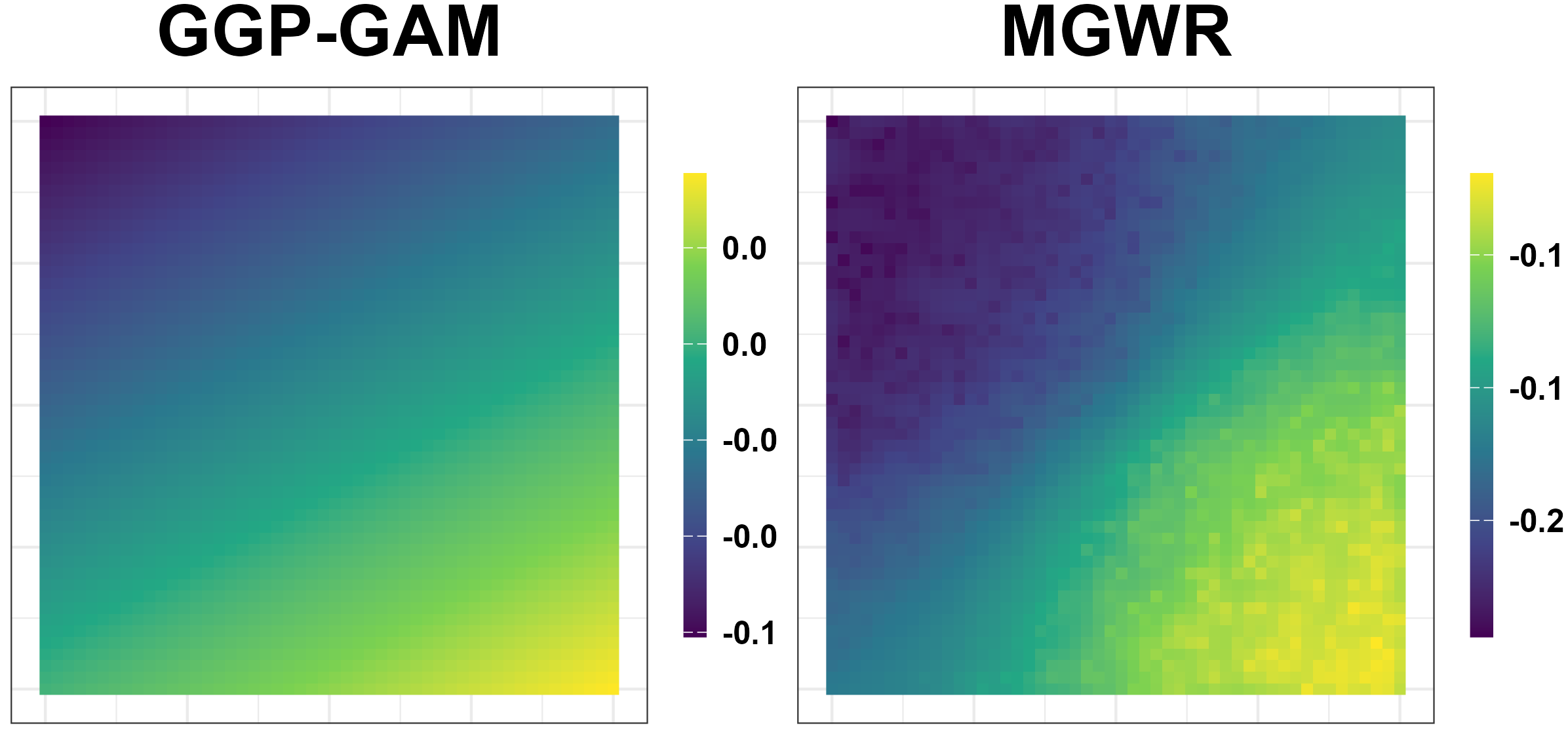
Simulation Results: Unreliable Spatial Patterns

• GGP-GAM and MGWR produce spurious spatial patterns.

Simulation Results: Performance Measures

SSGL-SVC is competitive in prediction and improves shrinkage of inactive surfaces, especially at smaller n.

Method	MSPE	MSE_1	MSE_0	MSE_{\text{avg}}
n=1000
Gaussian-SVC	1.18	0.78	0.85	0.81
BSGL-SVC	1.14	0.74	0.40	0.60
GGP-GAM	1.10	0.89	0.07	0.56
SSGL-SVC	1.10	0.68	0.12	0.46
n=10000
Gaussian-SVC	1.03	0.22	0.18	0.20
BSGL-SVC	1.03	0.20	0.13	0.17
GGP-GAM	1.02	0.15	0.04	0.10
SSGL-SVC	1.01	0.18	0.05	0.12

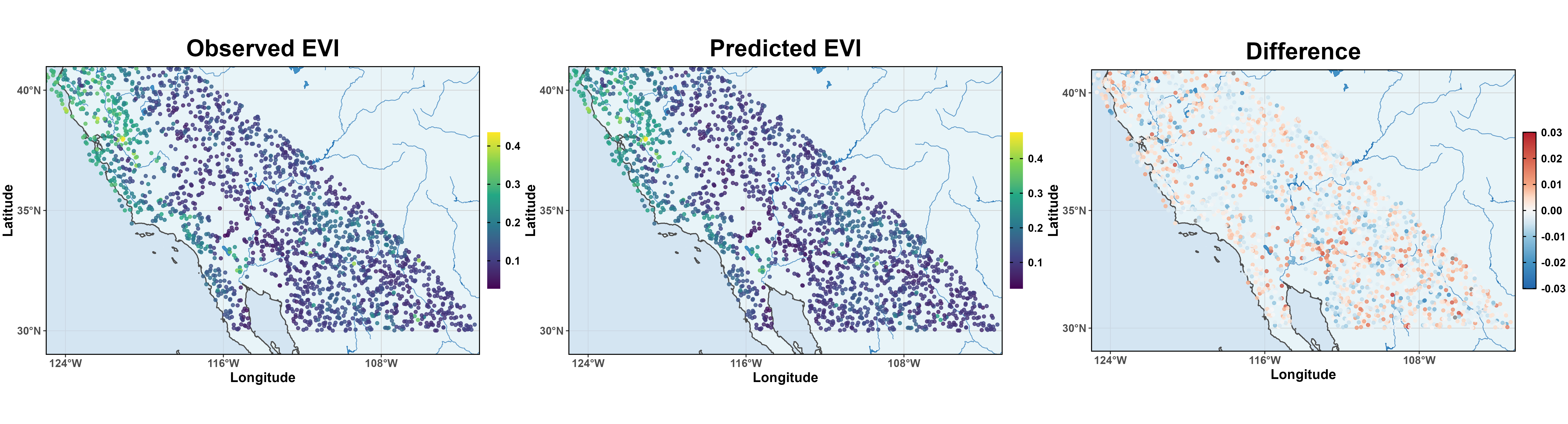
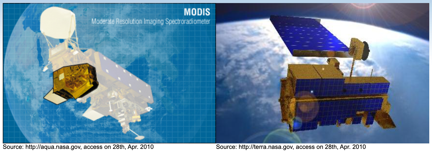
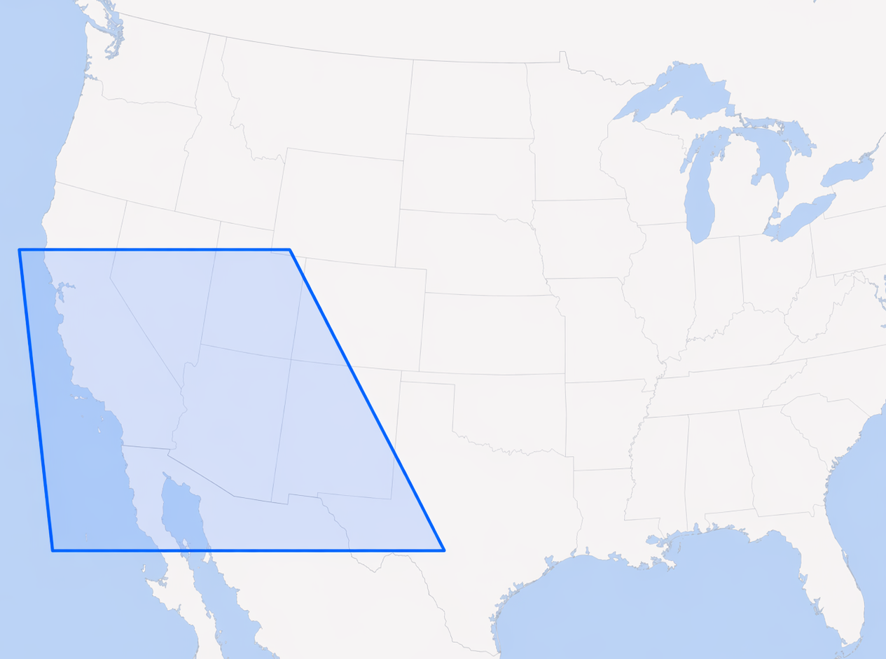
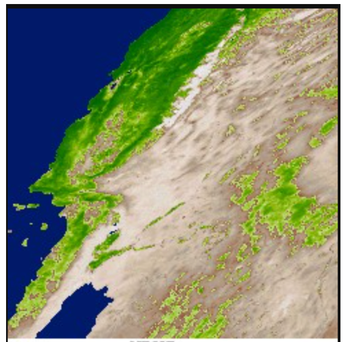
Real Data Application

• MODIS (Moderate Resolution Imaging Spectroradiometer) by NASA on the region 30°N-40°N latitude, 104°W-130°W longitude

• Response: Enhanced Vegetation Index (EVI) measuring vegetation greenness (Huete et al. 2002)

• 10 predictors:

  • Spectral Reflectance: Red, NIR, Blue, MIR
  • Ecosystem: GPP (amount of carbon through photosynthesis), LE (heat flux)
  • Satellite Observation Geometry: View/Sun zenith angle, Azimuth angle
  • Land Surface: LC Type4

Which predictors have spatially varying associations with EVI?

• Effects may differ across locations, so a global coefficient can be misleading
• The proposed method selects a parsimonious set of predictors and reveals their spatial patterns This real data example illustrates the practical value of the method. In this application, the scientific question is not only which predictors matter, but also whether their effects differ across space. The SSGL framework gives a parsimonious model and a more interpretable spatial story than a single coefficient model.

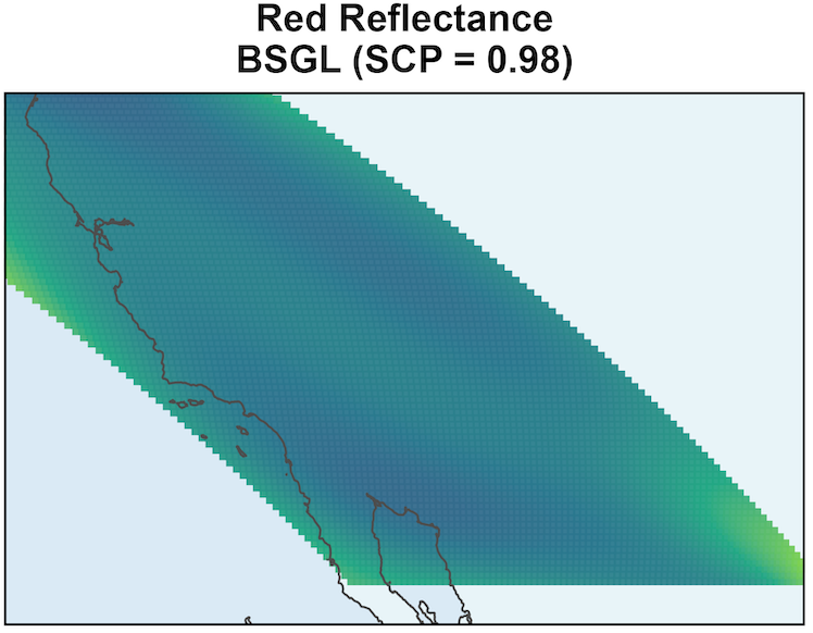
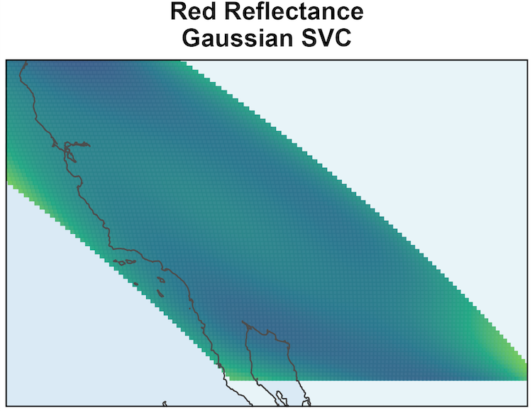
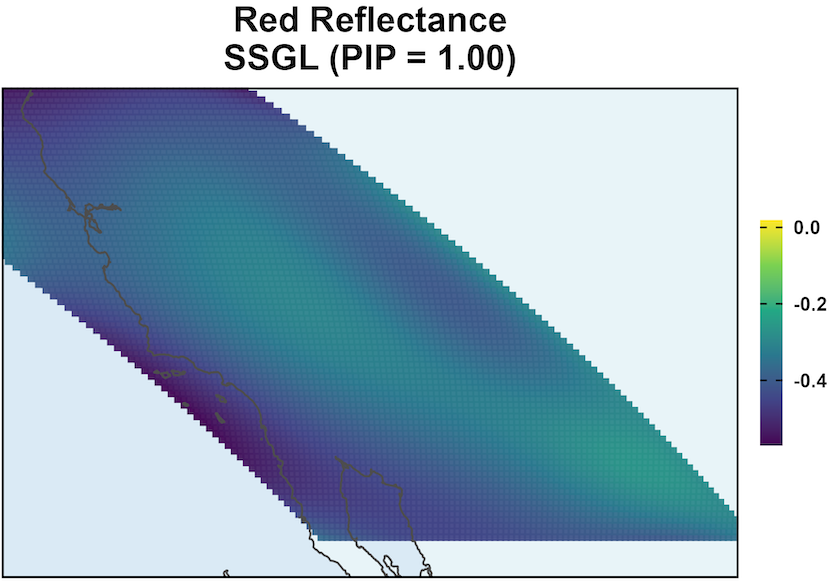
MODIS: Coefficient Surface and Selection

• SSGL-SVC leads to larger coefficient magnitudes.

• \text{PIP} \approx 1 shows Red Reflectance is associated with EVI, and it has a non-negligible coefficient surface.

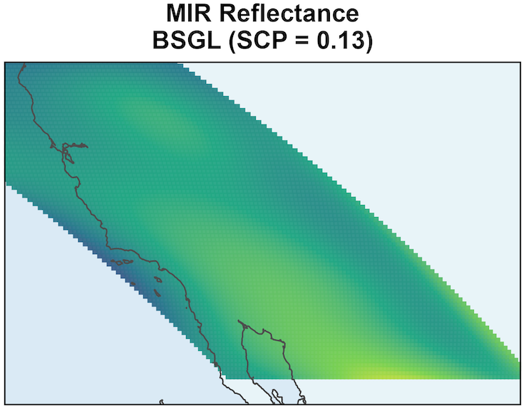
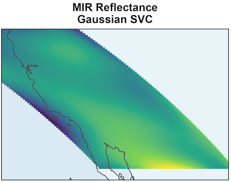
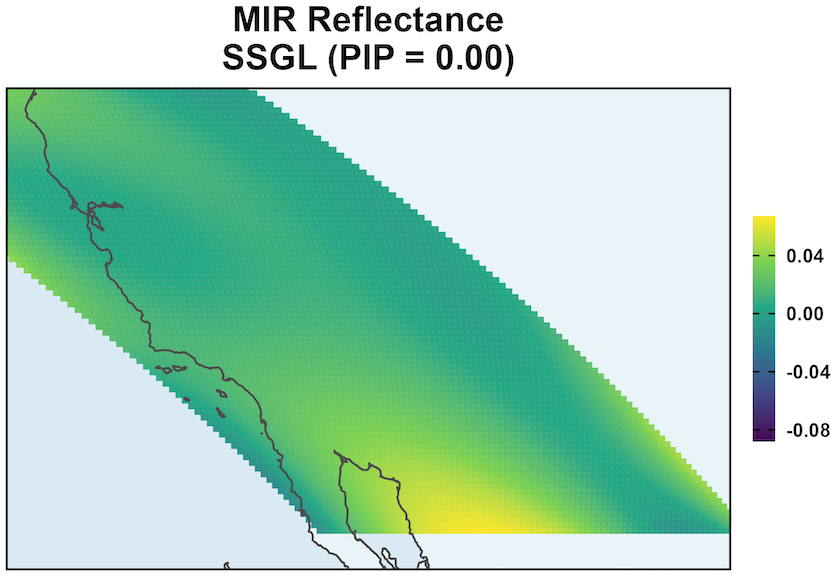
MODIS: Coefficient Surface and Selection

• SSGL-SVC shrinks coefficients more toward to 0 when the effect is negligible.

• \text{PIP} \approx 0 shows that given all other variables, MIR Reflectance’s effect is negligible.

• Remaining variation in \beta_{MIR}(s) is due to residual posterior uncertainty.

• The surface should not be interpreted as meaningful spatial signal.

MODIS: EVI Prediction

• Moran’s I verified that there is no spatial correlations in posterior residuals.

• Great MSPE 8.38 \times 10^{-5} and better than BSGL-SVC and Gaussian-SVC.

Take Home Messages

• We propose a novel SVC model
  • scalable via basis function approximation
  • variable selection via spike-and-slab group lasso
  • uncertainty quantification via Bayesian posterior probabilities

• Work in process and future work includes
  • spatiotemporal modeling: AR noises, \beta(s, t), \gamma_j(t), etc
  • Non-Gaussian responses: binary, counts, zero-inflated counts, etc
  • irregular or constrained space: smooth within region, abrupt across boundaries, within-surface local sparsity selection
  • scalable online learning: variational, EM + Laplace, NNGP / Vecchia / SPDE / sketching, etc

To conclude, our SSGL framework addresses an important gap in spatial modeling by combining flexible coefficient surfaces, groupwise selection, and Bayesian uncertainty quantification. The method works well in both simulation and real data settings, and we see it as a practical tool for modern spatial data analysis.

References

Babcock, Chad, Andrew O. Finley, John B. Bradford, Randall Kolka, Richard Birdsey, and Michael G. Ryan. 2015. “LiDAR Based Prediction of Forest Biomass Using Hierarchical Models with Spatially Varying Coefficients.” Remote Sensing of Environment 169: 113–27. https://doi.org/10.1016/j.rse.2015.07.028.

Banerjee, Sudipto, Alan E Gelfand, Andrew O Finley, and Huiyan Sang. 2008. “Gaussian Predictive Process Models for Large Spatial Data Sets.” Journal of the Royal Statistical Society Series B: Statistical Methodology 70 (4): 825–48.

Boehm Vock, Laura F., Brian J. Reich, Montserrat Fuentes, and Francesca Dominici. 2015. “Spatial Variable Selection Methods for Investigating Acute Health Effects of Fine Particulate Matter Components.” Biometrics 71 (1): 167–77. https://doi.org/10.1111/biom.12254.

Comber, Alexis, Paul Harris, and Chris Brunsdon. 2024. “Multiscale Spatially Varying Coefficient Modelling Using a Geographical Gaussian Process GAM.” International Journal of Geographical Information Science 38 (1): 27–47.

Eilers, Paul HC, and Brian D Marx. 1996. “Flexible Smoothing with b-Splines and Penalties.” Statistical Science 11 (2): 89–121.

Fotheringham, A Stewart, Wenbai Yang, and Wei Kang. 2017. “Multiscale Geographically Weighted Regression (MGWR).” Annals of the American Association of Geographers 107 (6): 1247–65.

Fotheringham, A. Stewart, Chris Brunsdon, and Martin Charlton. 2002. Geographically Weighted Regression: The Analysis of Spatially Varying Relationships. Wiley.

Gelfand, Alan E., Hyon-Jung Kim, C. F. Sirmans, and Sudipto Banerjee. 2003. “Spatial Modeling with Spatially Varying Coefficient Processes.” Journal of the American Statistical Association 98 (462): 387–96. https://doi.org/10.1198/016214503000170.

Guhaniyogi, Rajarshi, Cheng Li, Terrance D Savitsky, and Sanvesh Srivastava. 2022. “Distributed Bayesian Varying Coefficient Modeling Using a Gaussian Process Prior.” Journal of Machine Learning Research 23 (84): 1–59.

Hamm, Nicholas A. S., Andrew O. Finley, Martijn Schaap, and Alfred Stein. 2015. “A Spatially Varying Coefficient Model for Mapping PM10 Air Quality at the European Scale.” Atmospheric Environment 102: 393–405. https://doi.org/10.1016/j.atmosenv.2014.11.043.

Hipp, J. Aaron, and Nishesh Chalise. 2015. “Spatial Analysis and Correlates of County-Level Diabetes Prevalence, 2009–2010.” Preventing Chronic Disease 12: 140404. https://doi.org/10.5888/pcd12.140404.

Huete, Alfredo, Kamel Didan, Tomoaki Miura, E Patricia Rodriguez, Xiang Gao, and Laerte G Ferreira. 2002. “Overview of the Radiometric and Biophysical Performance of the MODIS Vegetation Indices.” Remote Sensing of Environment 83 (1-2): 195–213.

Ishwaran, Hemant, and J Sunil Rao. 2005. “Spike and Slab Variable Selection: Frequentist and Bayesian Strategies.”

Mu, Jingchao, Yifei Liu, Lynn Kuo, and Ming Hu. 2021. “Bayesian Variable Selection for the Cox Regression Model with Spatially Varying Coefficients with Applications to Louisiana Respiratory Cancer Data.” Biometrical Journal 63 (8): 1761–78. https://doi.org/10.1002/bimj.202000047.

Reich, Brian J., Montserrat Fuentes, Amy H. Herring, and Kelly R. Evenson. 2010. “Bayesian Variable Selection for Multivariate Spatially Varying Coefficient Regression.” Biometrics 66 (3): 772–82. https://doi.org/10.1111/j.1541-0420.2009.01333.x.

Roksvåg, Thea, Ingelin Steinsland, and Kolbjørn Engeland. 2022. “A Geostatistical Spatially Varying Coefficient Model for Mean Annual Runoff That Incorporates Process-Based Simulations and Short Records.” Hydrology and Earth System Sciences 26: 5391–5410. https://doi.org/10.5194/hess-26-5391-2022.

Scheipl, Fabian, Ludwig Fahrmeir, and Thomas Kneib. 2012. “Spike-and-Slab Priors for Function Selection in Structured Additive Regression Models.” Journal of the American Statistical Association 107 (500): 1518–32.

Shang, Zuofeng, and Murray K. Clayton. 2012. “An Application of Bayesian Variable Selection to Spatial Concurrent Linear Models.” Environmental and Ecological Statistics 19 (4): 521–44. https://doi.org/10.1007/s10651-012-0199-y.

Tibshirani, Robert. 1996. “Regression Shrinkage and Selection via the Lasso.” Journal of the Royal Statistical Society: Series B 58 (1): 267–88.

Wahba, Grace. 1990. Spline Models for Observational Data. Vol. 59. Philadelphia, PA: Society for Industrial; Applied Mathematics.

Wheeler, David C. 2009. “Simultaneous Coefficient Penalization and Model Selection in Geographically Weighted Regression: The Geographically Weighted Lasso.” Environment and Planning A 41 (3): 722–42. https://doi.org/10.1068/a40256.

Yuan, Ming, and Yi Lin. 2006. “Model Selection and Estimation in Regression with Grouped Variables.” Journal of the Royal Statistical Society: Series B 68 (1): 49–67. https://doi.org/10.1111/j.1467-9868.2005.00532.x.

Zhan, Qishi, Cheng-Han Yu, Yuchi Chen, Zhikang Dong, and Rajarshi Guhaniyogi. 2026. “Mapping Drivers of Greenness: Spatial Variable Selection for MODIS Vegetation Indices.” Journal of Agricultural, Biological and Environmental Statistics.